Model Inspector
Model parameters
Show explanationsGeneral parameters
Software:
PHOENIX 15.05.05C
Software package that was used to produce this model
Effective temperature [K]:
3600
Effective surface temperature in Kelvin
Surface gravity [log(CGS)]:
5.0
Base-10 logarithm of surface gravity in CGS
Stellar radius [Sun]:
0.3362
Effective radius of the star quantifying the departure from the plane-parallel approximation in solar radii
Outer pressure [log(CGS)]:
-3.0
Base-10 logarithm of the pressure (in CGS), defining the outer boundary of the atmosphere. The atmosphere above this level is not considered
Elemental composition
Hydrogen mass fraction, X [0..1]:
0.59693
Mass fraction of hydrogen (between 0 and 1)
Helium mass fraction, Y [0..1]:
0.40255
Mass fraction of helium (between 0 and 1)
Metals mass fraction, Z [0..1]:
0.00051
Mass fraction of metals (between 0 and 1)
Alpha enhancement, [a/H] [dex]:
0.0
Enhancement of Alpha elements (O, Ne, Mg, Si, S, Ar, Ca, Ti) in dex compared to solar
Elemental abundances, [A/M] [dex]:
Li
-03.00
Be
+00.00
B
+00.00
C
-00.65
N
+01.45
O
-00.10
F
+00.00
Ne
+00.00
Na
+00.00
Mg
+00.00
Al
+00.00
Si
+00.00
P
+00.00
S
+00.00
Cl
+00.00
Ar
+00.00
K
+00.00
Ca
+00.00
Sc
+00.00
Ti
+00.00
V
+00.00
Cr
+00.00
Mn
+00.00
Fe
+00.00
Co
+00.00
Ni
+00.00
Cu
+00.00
Zn
+00.00
Ga
+00.00
Ge
+00.00
As
+00.00
Se
+00.00
Br
+00.00
Kr
+00.00
Rb
+00.00
Sr
+00.00
Y
+00.00
Zr
+00.00
Nb
+00.00
Mo
+00.00
Ru
+00.00
Rh
+00.00
Pd
+00.00
Ag
+00.00
Cd
+00.00
In
+00.00
Sn
+00.00
Sb
+00.00
Te
+00.00
I
+00.00
Xe
+00.00
Cs
+00.00
Ba
+00.00
La
+00.00
Ce
+00.00
Pr
+00.00
Nd
+00.00
Sm
+00.00
Eu
+00.00
Gd
+00.00
Tb
+00.00
Dy
+00.00
Ho
+00.00
Er
+00.00
Tm
+00.00
Yb
+00.00
Lu
+00.00
Hf
+00.00
Ta
+00.00
W
+00.00
Re
+00.00
Os
+00.00
Ir
+00.00
Pt
+00.00
Au
+00.00
Hg
+00.00
Tl
+00.00
Pb
+00.00
Bi
+00.00
Th
+00.00
U
+00.00
Elemental abundances of metals in the atmosphere in dex with respect to metallicity-scaled and alpha-enhanced solar values, [A/M]
Iso-hydrogen, [X/H] [dex]:
-4.71:--
Abundances of hydrogen isotopes in dex compared to hydrogen-1. Deuterium:Tritium
Iso-carbon, [X/C] [dex]:
-1.95:--
Abundances of carbon isotopes in dex compared to carbon-12. Carbon-13:Carbon-14
Iso-nitrogen, [X/N] [dex]:
-2.43
Abundances of nitrogen isotopes in dex compared to nitrogen-14. Nitrogen-15
Iso-oxygen, [X/O] [dex]:
-3.42:-2.7
Abundances of oxygen isotopes in dex compared to oxygen-16. Oxygen-17:Oxygen-18
Stratification
Optical depth start:
-10.0
Base-10 logarithm of the shallowest optical depth (tau) in the calculation (upmost layer)
Optical depth end:
3.0
Base-10 logarithm of the deepest optical depth (tau) in the calculation (bottommost layer)
Number of layers:
128
Number of (spherical) vertical layers in the stratification
Reference wavelength [A]:
12750
Reference wavelength, at which the optical depth (tau) of a layer is defined
Convection modelling
Convection average:
0.5 mixing lengths
Width of the exponential averaging kernel applied to the square of convective velocity throughout the atmosphere
Mixing length [scale height]:
1.66
Convective mixing length in terms of local pressure scale heights
Convection depth:
-9.7
Base-10 logarithm of the minimum optical depth to consider convective energy transfer at
Convection cutoff:
0.01
Minimum fraction that convective energy transfer must contribute to the overall flux to be considered
Line selection
Line selection depth:
2.5e-05, 0.001, 0.01, 0.1, 1.0, 10.0, 100.0, 500.0
Optical depths, at which line selection is carried out
Select lines once:
Enabled
Select all relevant lines during the first iteration and maintain the same selection throughout
Atomic line window:
500.0 A
LTE Voigt atomic lines to be included are searched within this range around each wavelength sampling point
Molecular line window:
10.0 wavenumbers
LTE Voigt molecular lines to be included are searched within this range around each wavelength sampling point
Molecular band window:
1000.0 A
Molecular bands to be included are searched within this range around each wavelength sampling point
Gauss line window:
10.0 Doppler widths
LTE Gaussian lines to be included are searched within this range around each wavelength sampling point
Gauss atomic cutoff:
None
Minimum LTE atomic Gaussian line intensity (as a fraction of the continuum) to be considered in the calculation
Molecular band cutoff:
1.6
Minimum molecular band intensity (as a fraction of the continuum) to be considered in the calculation
Gauss molecular cutoff:
-6.0
Minimum LTE molecular Gaussian line intensity (as a fraction of the continuum) to be considered in the calculation
Voigt atomic cutoff:
-1.0
Minimum LTE atomic line intensity (as a fraction of the continuum) to be treated with a Voigt profile. Lower intensities may be treated with a Gaussian profile instead
Voigt molecular cutoff:
1.3
Minimum LTE molecular line intensity (as a fraction of the continuum) to be treated with a Voigt profile. Lower intensities may be treated with a Gaussian profile instead
Wavelength sampling
Wavelength start [A]:
1.0
Minimum wavelength in the requested spectrum output in angstroms
Wavelength end [A]:
9995000.0
Maximum wavelength in the requested spectrum output in angstroms
Maximum resolution:
27000
Maximum spectroscopic resolution in the requested spectrum output
Median resolution:
14212
Average spectroscopic resolution in the requested spectrum output
Non-Local Thermodynamic Equilibrium
NLTE treatment:
Enabled
When enabled, special NLTE treatment is applied to the lines that support it. Levels in full LTE regardless
NLTE Gauss window:
5.0 Doppler widths
NLTE Gaussian lines to be included are searched within this range around each wavelength sampling point
NLTE Lorentz window:
6000.0 Doppler widths or 8000.0 A
NLTE Lorentzian lines to be included are searched within this range around each wavelength sampling point
NLTE Lorentz sampling:
5 points from 5.0 to 1000.0
Wavelength offsets from the core, at which NLTE line profiles will be sampled in Lorentz widths
NLTE Gauss sampling:
5 points from 0.5 to 5.0
Wavelength offsets from the core, at which NLTE line profiles will be sampled in Doppler widths
NLTE special sampling:
3000
Selected NLTE lines are treated with special line profiles that will be sampled at this number of wavelength points
NLTE species:
HI, HeI, NaI, KI, LiI, CaI, CaII, RbI, CsI
List of species whose transitions receive NLTE treatment
Numerical methods and optimization
PP tables:
Enabled
Use precomputed partial pressure tables in the equation of state calculation
Switch-over depth:
0.5
Optical depth, below which the differential (as opposed to integral) form of energy conservation is used to calculate temperature corrections. See 2003ASPC..288...69D
dT=0 depth:
Disabled in final results
Base-10 logarithm of the optical depth, above which the temperature is assumed constant
Passive damping:
4
All temperature corrections are suppressed by this factor to avoid rapid oscillations in the structure between iterations at the expense of computation speed
Active damping:
Disabled
Anomalously large temperature corrections are detected and suppressed further in addition to the passive damping
Convection damping:
4
Additional passive damping in highly convective layers
Dust and clouds
Dust status:
Enabled
Provide a complete treatment of dust grains including their contribution to radiative transfer (opacity) and equation of state
Cloud status:
Disabled
Use the PHOENIX dynamical equilibrium cloud scheme ("Settl"). Otherwise, use the "Dusty" configuration.
Cloud coverage:
1.0
Fraction of the surface area covered with clouds
Settling EOS:
Disabled
Allow the abundances employed in calculating the equation of state to vary due to gravitational settling
Dust porosity [0..1]:
0.0
The porosity factor assumed in dust grains. The factor reduces the grain mass for the same grain size
Dust species:
51
Total number of dust species considered
Dust albedo [0..1]:
0.2
Average efficiency of radiation scattering (as opposed to absorption) by dust grains
Grain size distribution:
Log-normal
Functional form of the dust grain size distribution
Average grain size [log(cm)]:
-6.0
Base-10 logarithm of the average size of a dust grain around which the distribution is centered
Deviation in grain size [ln(cm)]:
1.0
Natural logarithm of the standard deviation in the grain size distribution
Grain size sampling:
12
Number of points in the dust grain size distribution sampling
Miscellaneous
Turbulent velocity [km/s]:
0.326389 + convection
Turbulent velocity in km/s. If indicated, the value may be increased in highly convective layers
Atomic albedo [0..1]:
0.0
Efficiency of radiation scattering (as opposed to absorption) by atomic lines
Molecular albedo [0..1]:
0.0
Efficiency of radiation scattering (as opposed to absorption) by molecular lines
Molecules status:
Enabled
Include molecules in the PHOENIX calculation
Line blanketing:
Enabled
Include LTE line blanketing in the radiative transfer
Saumon-Chabrier EOS:
Enabled
Use the Saumon-Chabrier H/He model in the equation of state calculation
EOS species:
343:74:117
Total number of species considered in the equation of state. Gaseous:liquid:crystalline
Synthetic Spectrum

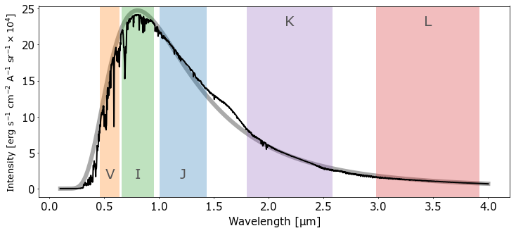
Figure 1. Synthetic spectrum of the atmosphere. Isotropic intensity per unit surface area of the star per unit wavelength per unit solid angle. Shown in light gray is the blackbody spectrum
for the same effective temperature as the model (3600 K). Selected optical and near-IR photometric bands are highlighted.
Atmosphere Structure

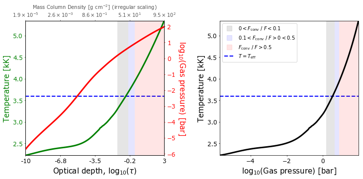
Figure 2. Left: temperature (green) and gas pressure (red) as functions of the optical depth throughout the model atmosphere. Temperature is shown on a linear scale, while both optical depth
and pressure are logarithmic. For reference, an alternative horizontal scale is provided with markings in terms of mass column density instead of optical depth. Note that the alternative
scale corresponds directly to the optical depth scale and may therefore be irregular (i.e. neither logarithmic nor linear). Right: temperature as a function of pressure. The effective
temperature of the model (3600 K) is shown in blue in both plots. Strongly convective regions are highlighted.
Solution Convergence

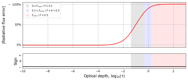
Figure 3. Percent flux error in the model as a function of optical depth. The vertical axis is logarithmic and shows the absolute value of the error, while the sign is provided as a separate
plot. Temperature corrections in each iteration are carried out to minimize the error; however, some residuals will remain due to (1) incomplete/inaccurate physics, (2) numerical failures
and (3) insufficient number of iterations. For ATLAS models, flux errors below 1% are typically expected throughout the entire atmosphere in a well-converged model. At low temperatures,
flux errors up to 10% are sometimes tolerated in localized regions. For PHOENIX models, errors of a few percent are expected in radiative layers. In highly convective regions, the error
estimate is not representative of the model convergence and may rise to arbitrarily large values. Well-converged models usually show a smooth transition between the two regimes and are
free of oscillations.